Toggle navigation

.md .pdf

repository

Contents

Tutorial

This tutorial consist of two parts: a relatively simple analysis of a very small alignment file avaliable in repository, and a larger and more real life analysis of the Kap Copenhagen dataset.

Simple Analysis

Input data

To run the full suite of commands, i.e. the LCA and fits, metaDMG requires the following input files:

1. An aligment file (or a directory containing multiple alignment files).

2. A names file, which contains the names of the different accessions in the database.

3. A nodes file, which contains the relationship between the different accessions in the database (the graph structure, so to speak).

4. A acc2tax file, which is the conversion between accesion number and the tax ID.

To make the introduction to metaDMG easy, metaDMG is by default shipped with a small data directory containing these.

These files can be loaded by running the following command:

$ metaDMG get-data --output-dir raw_data

where raw_data is the output directory where you want to store the files.

Config

Now that the we have the raw data, we can start running metaDMG. For ease of use, metaDMG is structured such that we first need to generate a config file which contains all of the options that the LCA and fits require. To compare two different analysis, one simply need to compare the config files. As such, the config file can thus be seen as all the relevant metadata.

metaDMG config should have sensible defaults. The full specification of the avaliable options can be found either by running metaDMG config --help or for a more thorough explanation, see here.

Since the data we have in this example is quite small, we want to run the full Bayesian analysis. As such, we generate the following config file:

$ metaDMG config raw_data/alignment.sorted.bam \
    --names raw_data/names-mdmg.dmp \
    --nodes raw_data/nodes-mdmg.dmp \
    --acc2tax raw_data/acc2taxid.map.gz \
    --custom-database \
    --bayesian

Most of the options should be quite self-explanatory. --bayesian indicates that we want to run the full Bayesian model, which is slower than the faster, approximate model that we use by default. The --custom-database flag is needed since this database is not the full NCBI one.

After running this command, you should notice a new file in your directory: config.yaml. This is a normal .yaml file which can be opened and edited with your favorite text editor. In case you wanted to call the config file something different, you can add --config-file config_simple.yaml.

The same as above can also be done more visually by using the config-gui command:

$ metaDMG config-gui

Just remember to check the relevant boxes off and save a config file. In case you are missing any mandatory fields, it should pop up and warn you automatically.

Compute

Now that we have generated a config file with all of the necessary parameters, we can start the actual computation. This is done by running:

$ metaDMG compute

or, in the case of another name for the config file:

$ metaDMG compute config_simple.yaml

When you enter the command, metaDMG will first parse the config file and extract the relevant parameters for the LCA. The C++ part of the program will perform the LCA of the reads in the alignment file and output its intermediary files in {output-dir}/lca/ (data/lca by default). This step can take a while on real datasets.

We then load these files and turn them into a mismatch matrix (XXX link here) in a pandas dataframe. Now, having a mismatch matrix for each tax ID, we fit each of these independently. Since we added the --bayesian flag previously, we perform the full, Bayesian analysis in addition to the fast, approximate version. For more information, see XXX link here to information. This step can also be quite slow on real datasets, which is also why we do not do this by default.

Finally, after the fits are done, we merge the fit results with some additional information from the mismatch matrices and save the results to disk in {output-dir}/results/ (data/results by default). For a more concrete overview of all of the variables saved as results, see XXX.

Visualisation

Now, after we have computed the results, it’s time to analyse them. Instead of looking at static pdf plots, we include an interactive dashboard with metaDMG. This easy to start, you just simply run:

$ metaDMG dashboard

or, in the case of another name for the config file:

$ metaDMG dashboard config_simple.yaml

Overview plot

The command above will open a page in web browser automatically where you will see the following image:

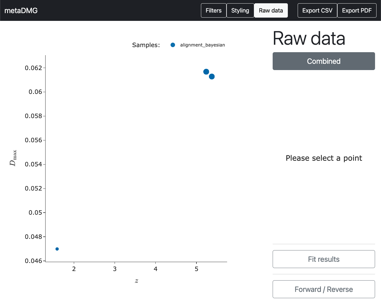
In the middle of the page, we see the overview plot. This shows the amount of damage, \(D\), on the y-axis and the significance, \(Z\), on the x-axis. In this case, we see three blue dots; one single dot per tax ID.

In general, we want a large amount of damage along with a high significance to believe that the related data is significantly ancient. In this case, the two points in the upper right seem like good potential candidates.

Hover info

To extract more concrete information about the individual tax IDs (points in the plot), we can hover the mouse on top of the point:

Here we have hovered the mouse on the tax ID 711 which is the Lactobacillales order. Below the tax information, we can see the fit results, in particular the position-dependent damage-rate, \(q\), the fit concentration \(\phi\) and the correlation between \(A\) and \(c\), \(\rho_{Ac}\), along with the significance and damage amount.

In this small analyses, we ran the full Bayesian model. In the more general case where this would be too time consuming, we would only have the MAP results. These are show below. In this case, the MAPsignificance is measured by the MAP significance \(Z_\text{MAP}\). Note the strong correspondence between the Bayesian fit results and the approximate MAP results.

In the buttom of hover square, we see the count information. This shows, that this tax ID consisted of \(22.5 \times 10^3\) individual reads with the same number of alignments (indicating very little amount of overlap between the references in this case). The k sum total is the total number of \(C \rightarrow T\) transistions across all reads at all positions (and \(G \rightarrow A\) for the reverse strand). N sum total is the total number of \(C\) to anything, \(C \rightarrow X\), across all reads at all positions (and \(G \rightarrow X\) for the reverse strand).

Raw data plot

So now we have managed to extract the fit results of the specific tax ID. However, we might still be a bit sceptical about these estimates that a stranger on the internet claims to be important. To refute the scepticism, the raw data that the fit was based on can be shown by clicking on the point (instead of only hovering on it).

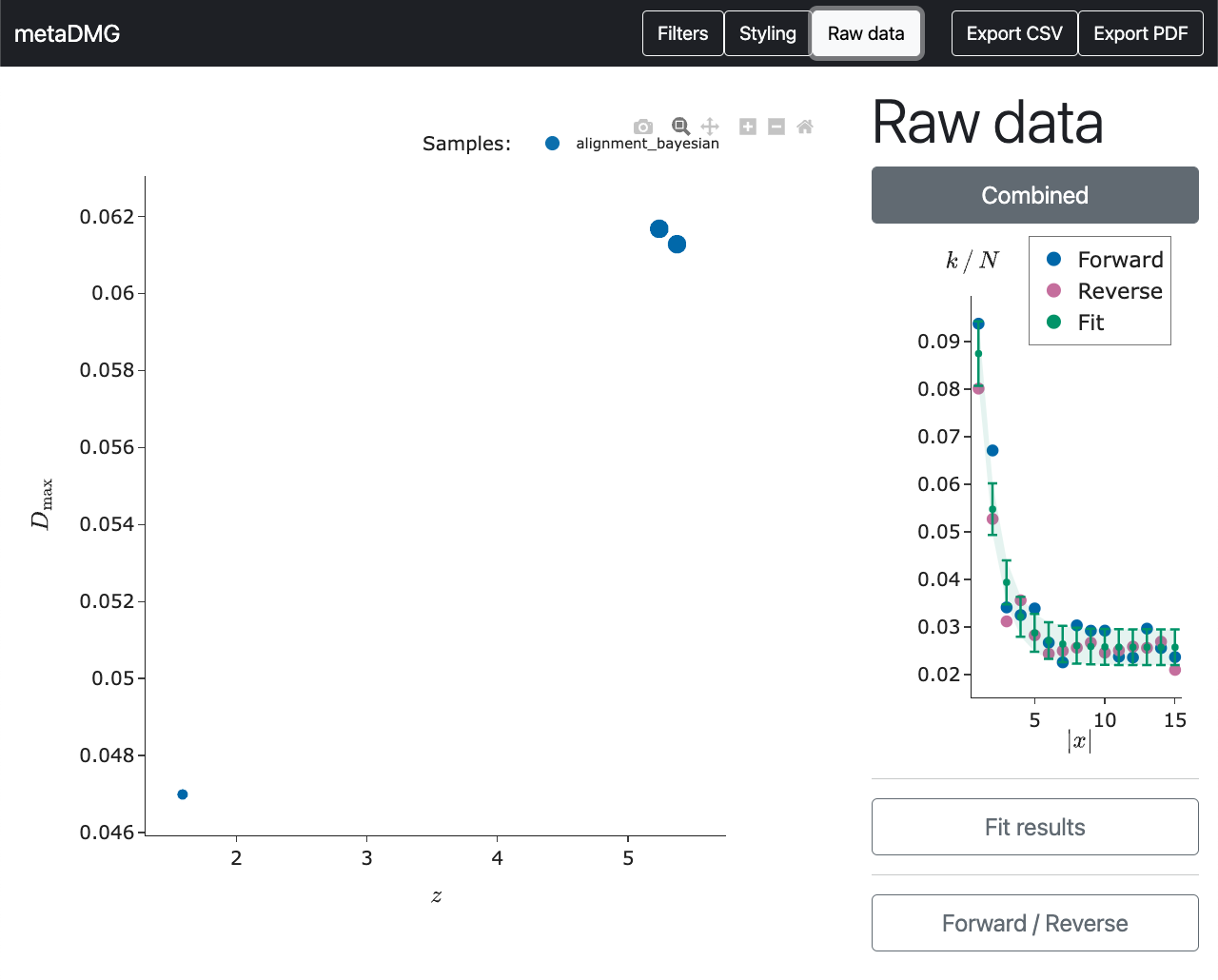
In this plot, the position dependent frequency of the \(C \rightarrow T\) transitions are shown in blue dots and the \(G \rightarrow A\) transitions in red. The green curve is the fit and the dashed area shows the \(1\sigma\) (68%) confidence interval of the fit.

We see that damage frequency starts at around 0.085 and then drops to about 0.025. This is an elevated amount of damage of about 0.06 in the beginning of the read compared to the asymptotic value, which is exactly what \(D\) explains. Similarly see a quite clear trend in the data; the visual appearance of the data matches the quantitative fit results.

We can compare this to the data in the bottom left of the overview plot.

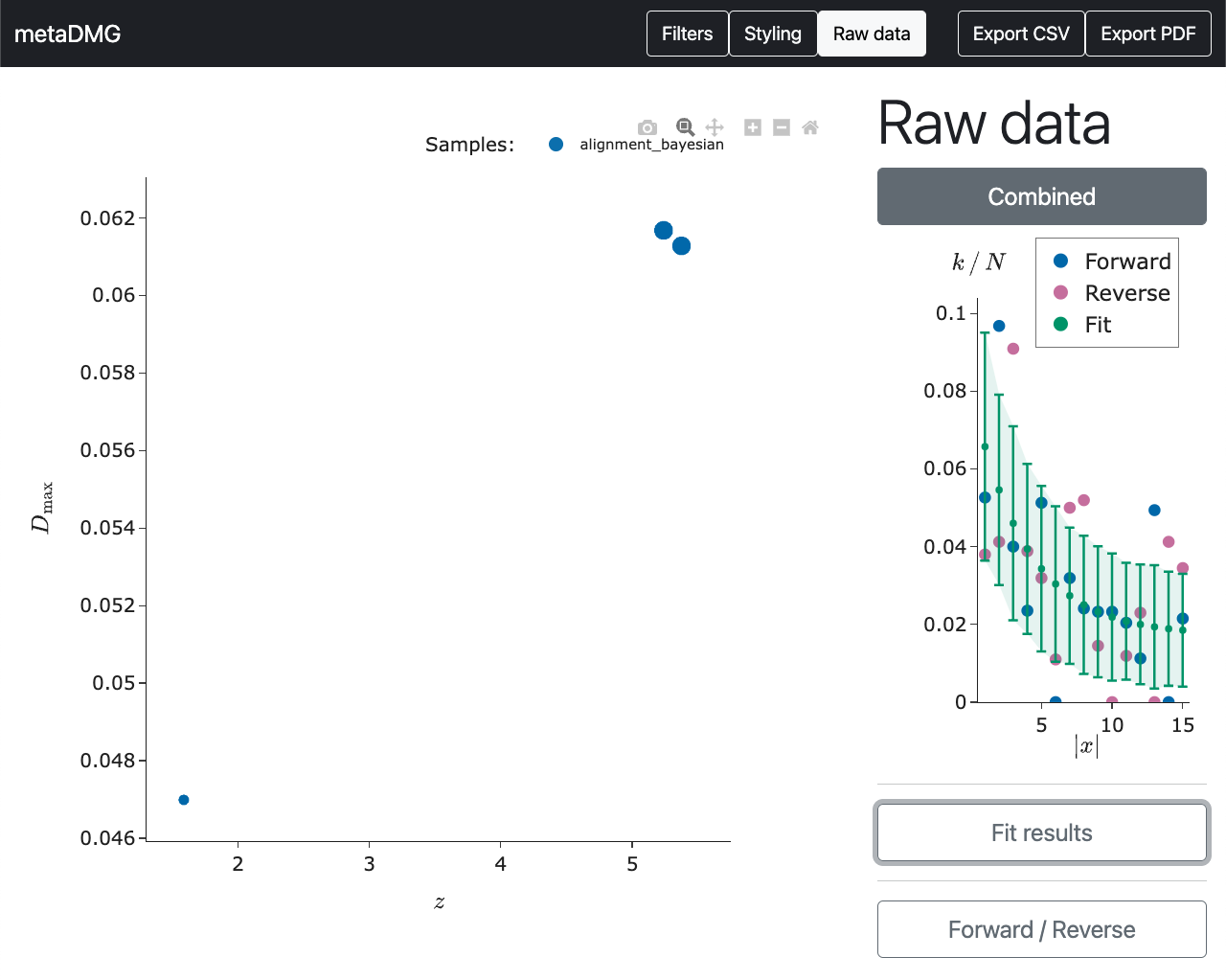
Here we see that there does seem to be some damage in this tax ID, although the data is a lot more noisy and scattered around. This is also why the significance, \(X\), is a lot smaller than it is for the previous tax ID.

Export CSV

If we wanted to export the results to a CSV file for further analysis, we can press the Export CSV button in the top right.

This is also possible through the command line without opening the dashboard:

$ metaDMG convert --output results_as_csv.csv

or, in the case of another name for the config file:

$ metaDMG convert config_simple --output results_as_csv.csv

Export PDFs

If we wanted to export the plots to a PDF file, we can press the Export PDF button in the top right. This will generate a single PDF file which contains both the overview plot and the individual raw data plots.

This is also possible through the command line without opening the dashboard:

$ metaDMG plot --output plots.pdf

or, in the case of another name for the config file:

$ metaDMG plot config_simple --output plots.pdf

Kap Copenhagen

metaDMG is also used in more advanced cases using real data, compared to the small, simulated example above. It is e.g. used in the Kap Copenhagen analysis, Kap K in short.

This analysis is based on dozens of samples from Northern Greenland, each more than 2 million years old. As such, they are expected to have a high degree of damage.

The overall workflow is the same as previously; generate a config file, compute it, and visualize the results.

Config

In this case we have all of the alignments file in a single folder on the server. Therefore, we take advantage of the fact that metadDMG config allows for not only running on single samples, but also multiple samples (or a directory of samples):

$ metaDMG config raw_data/*.bam \
    --names raw_data/names.dmp.gz \
    --nodes raw_data/nodes.dmp.gz \
    --acc2tax raw_data/ combined_taxid_accssionNO_20200726.gz \
    --parallel-samples 3 \
    --cores-per-sample 2 \
    --config-file config_KapK.yaml

Here we name the output config file config_KapK.yaml to be able to differentiate it from the previous one. On purpose, we do not run the full Bayesian model since the each sample file contains reads mapping to too many different tax IDs for it to be computationally feasible; as such, we use the fast, approximative model.

To further speed the process up, we run 3 samples in parallel and allow each of the samples to use 2 cores, i.e. using a total of up to \(3 \times 2 = 6\) cores. The --cores-per-sample does only affect the fitting part of the pipeline, not the LCA. In some cases it is the LCA that is the time consuming part and in others it is the fits, so change --parallel-samples and --cores-per-sample to fit your needs. For a visual explanation of this, the workflow diagram below might be helpful:

flowchart LR start(metaDMG) start --> A start --> B start --> C subgraph subgraph_A [Sample A] A(LCA) --> A1(Fit) & A2(Fit) --> A3(Merge) end subgraph subgraph_B [Sample B] B(LCA) --> B1(Fit) & B2(Fit) --> B3(Merge) end subgraph subgraph_C [Sample C] C(LCA) --> C1(Fit) & C2(Fit) --> C3(Merge) end A3 & B3 & C3 --> D(Results)

Compute

Now for the easy, but time consuming, part of the pipeline: the actual computation. This is simply by running the following command:

$ metaDMG compute config_KapK.yaml

We try to only print the most important information to the screen, but more information can be found in the log file at logs/.

Dashboard

After the computations are finished, we want to see the results. We can either copy the entire data/results/ directory from the server to our local computer, or we can run the actual dashboard on the server and then connect to it via SSH, thus circumventing the need for any local installation of metaDMG at all.

We start the dashboard:

$ metaDMG dashboard config_KapK.yaml --server

The --server option tells the dashboard that it should open in the background. In case you run into the following error: OSError: [Errno 98] Address already in use, it can help by changing the port by adding --port 8060.

We can now connect to it through an SSH connection. This depends on your server setup, but in our case we connect to our server through a jumphost:

flowchart LR start(LOCAL) --> jump("USER1@JUMPHOST") --> server("USER2@SERVER")

With this setup, we can connect in the following way (on our own, local machine!):

$ ssh -N -J USER1@JUMPHOST USER2@SERVER -L 8050:127.0.0.1:8050

where you change the USER1, JUMPHOST, USER2, and SERVER according to your own setup. Note that if you changed the port on the server, you also have to change it here.

We can now open a browser on our own, local computer and go to the following address: http://0.0.0.0:8050/ where the dashboard will be running live.

previous

Getting started

next

Command Line Interface