Dashboard
Contents
Dashboard
The dashboard provides an interactive visualisation of the results from metaDMG. You can use it locally by running:
$ metaDMG dashboard
or, in the case of another name for the config file:
$ metaDMG dashboard config_simple.yaml
For a short introduction on how to run it on a server and use a local browser, see the tutorial on the Kap K dashboard.
In case you just want a small preview of the dashboard, you can also use the following live dashboard.
Overview plot
When you open the dashboard, you will see the following:
In the middle of the page, we see the overview plot. This shows the amount of damage, \(D\), on the y-axis and the significance, \(Z\), on the x-axis. In this case, we see three blue dots; one single dot per tax ID.
In general, we want a large amount of damage along with a high significance to believe that the related data is significantly ancient. In this case, the two points in the upper right seem like good potential candidates.
Hover info
To extract more concrete information about the individual tax IDs (points in the plot), we can hover the mouse on top of the point:

Here we have hovered the mouse on the tax ID 711 which is the Lactobacillales order. Below the tax information, we can see the fit results, in particular the position-dependent damage-rate, \(q\), the fit concentration \(\phi\) and the correlation between \(A\) and \(c\), \(\rho_{Ac}\), along with the significance and damage amount.
In smaller analyses, the full Bayesian model can be used (which is recommended). In the more general case where this would be too time consuming, we would only have the MAP results. In this case, the significance is measured by the MAP significance \(Z_\text{MAP}\).
In the bottom of the hover square, we see the count information. This shows, that this tax ID consisted of \(22.5 \times 10^3\) individual reads with the same number of alignments (indicating very little amount of overlap between the references in this case). The k sum total is the total number of \(C \rightarrow T\) transitions across all reads at all positions (and \(G \rightarrow A\) for the reverse strand). N sum total is the total number of \(C\) to anything, \(C \rightarrow X\), across all reads at all positions (and \(G \rightarrow X\) for the reverse strand).
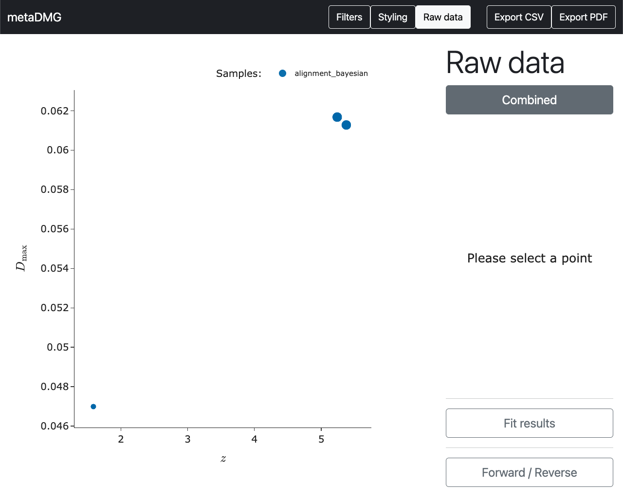
Raw data plot
The hover square shows the overall information. However, we might want to see even more information. The raw data that the fit was based on can be shown by clicking on the point (instead of only hovering on it).
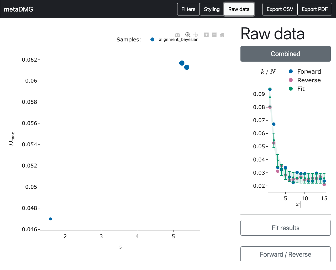
In this plot, the position dependent frequency of the \(C \rightarrow T\) transitions are shown in blue dots and the \(G \rightarrow A\) transitions in red. The green curve is the fit and the dashed area shows the \(1\sigma\) (68%) confidence interval of the fit.
Fit results
If we click on the Fit results button, we get the same information as in the hover square along with some extra information. If one has run the full Bayesian model, this is where we can see both the Bayesian results and the MAP results. In the botton, the full taxonomic path is shown.
Forward / Reverse
The Forward / Reverse button shows the individual fits to the forward and reverse strand (a MAP fit). The asymmetry variable in the fit result is based on this.
Filters
If we hide the Raw Data pane by clicking on it and instead show the Filters pane by clicking on it, we see the following:
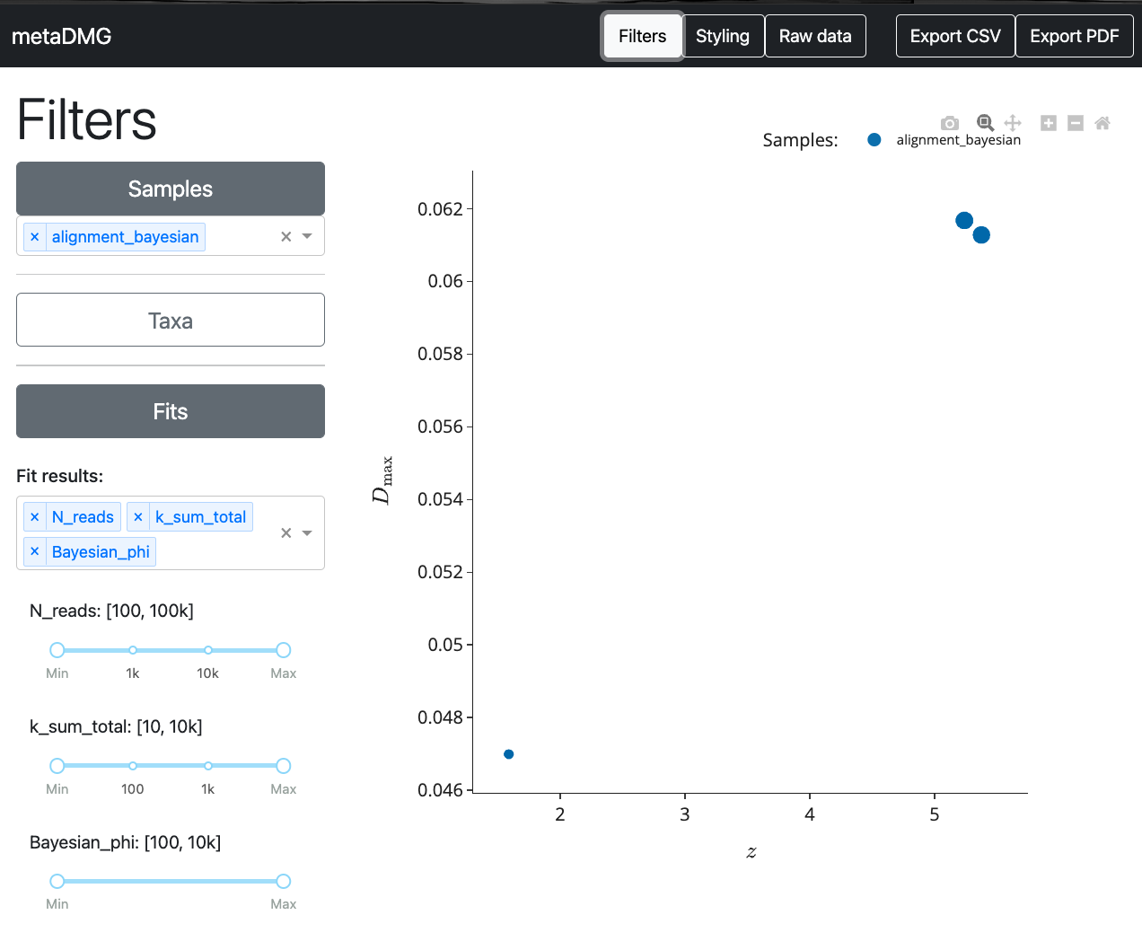
This is where we can apply different selection criteria and filters to the metaDMG results.
Samples
The Samples button allow one to select which samples the dashboard includes in the plots. In this way, one can choose to focus on specific samples. Notice the Select All option in the dropdown menu.
Taxa
The Taxa button allow one to select which samples the dashboard includes in the plots.
The Specific taxas dropdown menu allow one to focus on specific taxas or tax IDs. This could e.g. be Lactobacillales or 711.
The Taxonomic path contains is a more general filter, that allows one to select e.g. all taxa that are within the bacteria superkingdom by writing Bacteria or within the fusobacteria class by writing Fusobacteriia.
Fits
The Fits button allow one to apply specific selection criteria based on the fit results. The top dropdown allows one to select specific variables to cut on and a slider related to that variable is then automatically added below.
An example could be if one only wants to inspect fits with a very large number of reads in them. The you would slide the left part of the N_reads slider to 1k which would correspond to setting the minimum number of reads to 1000.
Styling
If we hide the Filters pane by clicking on it and instead show the Styling pane by clicking on it, we see the following:
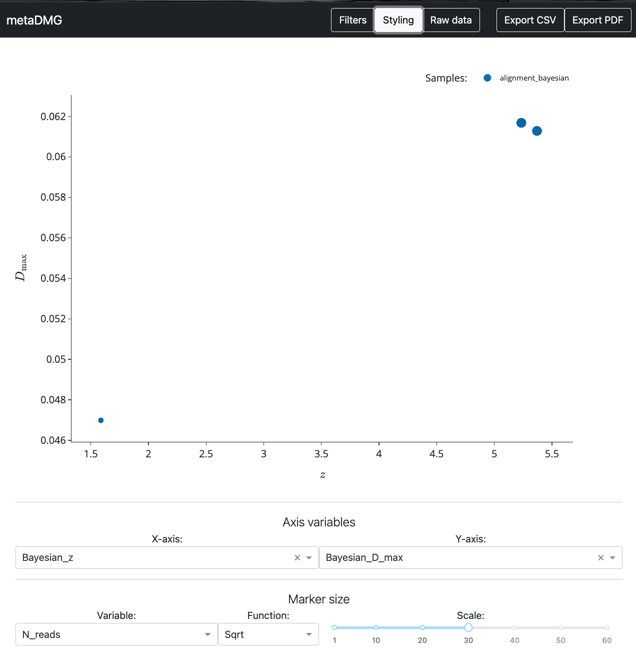
This allows to go deeper into the fit results and explore more advanced relationships between the variables. If one e.g. changes the x-axis to show MAP_damage, it is possible to visually compare the two estimates of \(D\); the MAP one and the Bayesian one.
All of the points in the dashboard are sized according to the number of reads. This can be changed in the Variable dropdown. By default, they are sized according to the square root of this variable; this can also be changed in the Function dropdown. Finally, a relative scaling is also positive in the Scale slider.
Export CSV
If we wanted to export the results to a CSV file for further analysis, we can press the Export CSV button in the top right.
This is also possible through the command line without opening the dashboard:
$ metaDMG convert --output results_as_csv.csv
or, in the case of another name for the config file:
$ metaDMG convert config_simple --output results_as_csv.csv
Export PDFs
If we wanted to export the plots to a PDF file, we can press the Export PDF button in the top right. This will generate a single PDF file which contains both the overview plot and the individual raw data plots.
This is also possible through the command line without opening the dashboard:
$ metaDMG plot --output plots.pdf
or, in the case of another name for the config file:
$ metaDMG plot config_simple --output plots.pdf